Singularities with Two Loops

Consider the system $\Omega = \{ i_+, j_+, k, i_-, j_- \}$ of five binary variables, interacting along
two triangular loops $i_+ j_+ k$ and $i_-j_-k$ meeting in $k$.

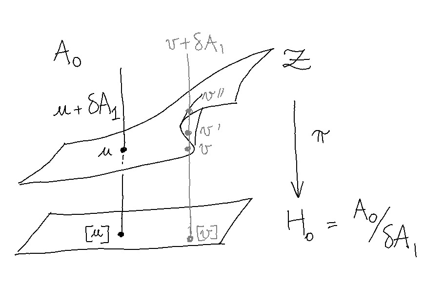
The submanifold ${\cal Z} \subseteq A_0$ of consistent potentials, fixed by diffusion, is not everywhere transverse to the image $\delta A_1 \subseteq A_0$ of heat fluxes. It may therefore happen that the homology class $[u] = u + \delta A_1$ of a potential $u \in A_0$ intersects the equilibrium surface $\mathcal Z$ more than once.

The singular subspace ${\cal S_1} \subseteq {\cal Z}$, along which the intersection of $T {\cal Z}$ with $\delta A_1$ is of dimension $1$, is here a codimension $1$ analytic submanifold of ${\cal Z}$.

Cusp and Singularities

For every $u \in {\cal S_1}$, there exists a unit flux term $\delta \varphi \in \delta A_1$ spanning $T_u {\cal Z} \cap \delta A_1$.

Singular equilibria are generically unstable, so that perturbing $u$ in the direction of $ \pm \delta \varphi$ may lead to another distant equilibrium $u’ \in {\cal Z} \cap [u]$ under diffusion. Along a path in ${\cal S_1}$, it may furthermore happen that the two homologous equilibria $u \sim u’$ meet, in which case $u$ is called a cusp.

In the plots below, such a path in ${\cal S_1}$ is observed: each trace corresponds to a different diffusion starting from a perturbed initial condition $u_0 = u + \delta \varphi$, where $\delta \varphi$ spans $T_u {\cal Z} \cap \delta A_1$ and $u$ follows a smooth path leaving from the cusp.

Distance away from $u$

In the acyclic case, diffusion is ensured to converge to a single equilibrium within any given homology class $[u] = u + \delta A_1$. Hence ${\cal Z}$ is attractive and perturbing $u \in {\cal Z}$ by a flux term $\delta \varphi$ always leads back to $u$.

By contrast, the plot below shows that equilibria within $[u]$ for $u \in {\cal S_1}$ are generically multiple: as $u$ moves away from the cusp, the homologous equilibrium $u’ = \lim_{t \to \infty} u_t$ parts with $u$.

Distance away from ${\cal Z}$

The stationary manifold ${\cal Z}$ is defined by the effective consistency constraints ${\cal D}(U) = 0$, where $U = \zeta \cdot u$ denotes the local hamiltonians associated to a potential $u$. The norm of ${\cal D}(U)$ hence represents an amount of inconsistency and a distance away from ${\cal Z}$.

In the acyclic case, this amount of inconsistency seems to always follow an exponential decay under diffusion.

By contrast, the plot below shows integral curves starting relatively close from the stationary manifold that locally flow away from ${\cal Z}$, until they hit another stationary layer folded across $\delta A_1$.

The Singular Subspace

The singularity condition $\delta \varphi \in {\rm Ker}(\nabla_u \circ \zeta) = T_u {\cal Z}$ yields conservation equations of the form:

for all edge-vertex pair $jk \to k$ in the degree-one nerve of $X$. Denoting by $M : A_1 \to A_1$ the operator $1 - (\nabla_u \circ \zeta \circ \delta)$, the above system of equations derives from $\varphi = M(\varphi)$, having non-trivial solutions if and only if $1$ is an eigenvalue of $M$.

Parameterising ${\cal Z}$

Denote by ${\mathbb E}^{jk \to k} = {\mathbb E}^{jk}[-|k]$ the conditional expectation operator, orthogonal projection of $A_j$ onto $A_k$ viewed as subspaces of $A_{jk}$, for the metric induced by local Gibbs states.

Given orthonormal bases of $(1_j, v_j)$ and $(1_k, v_k)$ of $A_j$ and $A_k$, conditional expectations take a diagonal form:

where the eigenelements $\lambda_{jk}$ and $v_j$ are given by:

and $p_{jk}$ is the local Gibbs state, normalising the Gibbs density ${\rm e}^{-U_{jk}} = {\rm e}^{-u_{jk} - u_j - u_k}$. The above remark stands for any pair of binary variables $(x_j, x_k) \in \{ \pm 1 \}^2$.

Furthermore introducing local magnetic fields $b_j = - {1 \over 2} \ln(p_j^+ / p_j^-)$, by the real numbers $\{ b_j , \lambda_{jk} \}$ for any graph of binary variables, with:

translating positivity constraints in the space of parameters, while $\lambda_{jk} \leq 1$ by construction.

Parameterising ${\cal S_1}$

One may show that ${\cal S_1}$ is defined by a quadratic equation on loop eigenvalues:

where $\Lambda^{\pm} = \lambda_{k i^\pm} \, \lambda_{i^\pm j^\pm} \, \lambda_{j^\pm k}$ is the non-trivial eigenvalue of the loop operator ${\rm L}^\pm : A_k \to A_k$ obtained by composing conditional expectations:

Deriving ($\ref{hyperbola}$) from the conservation equations ($\ref{conservation}$) is left as an exercise to the reader: using the previous parameterisation of ${\cal Z}$, conditional expectations act as multiplications by scalars and lead to computations somewhat reminiscent of Kirchhoff’s laws on electric circuits.

A few more efforts are required to write $\varphi \mapsto M(\varphi)$ in diagonal form, to a parameterise a current $\varphi \in A_1$ singular as soon as equation $(\ref{hyperbola})$ holds.

Note that only the largest eigenvalue of $M$ may reach $1$, so that the stratified space \({\cal S} = \bigcup_k {\cal S}_k\) is indeed a codimension \(1\) analytic submanifold of \({\cal Z}\), with \({\cal S} = {\cal S}_{1}\) and \({\cal S}_2 = {\cal S}_{3} = \dots = \varnothing\).

Tuning parameters

The controls below are mapped to points in ${\cal Z}$, with fields $b_i$ in red and couplings $\lambda_{ij}$ in green.

The yellow square $]-1, +1[^2$ describes possible values for the pair $(\Lambda^+, \Lambda^-)$, in which ${\cal S_1}$ projects to the hyperbola depicted in blue.

The two green triangles then describe logarithmic couplings on each loop, which by definition of the loop eigenvalue $\Lambda^\pm$ should solve:

Note that we assume positivity of each $\lambda_{ij}$ : as $\Lambda \in ]0, 1[$ no coupling on the loop may vanish, while reverting the sign of two adjacent couplings $\lambda_{ij}$ and $\lambda_{jk}$ may be seen equivalent to exchanging the “up” and “down” states $|+\rangle$ and $|-\rangle$ on the $j$ vertex. Therefore ${\cal S_1}$ is not connected in ${\cal Z}$, with $({\mathbb Z}/2 {\mathbb Z})^5$ acting on its $8$ diffeomorphic connected components.

The first red control describes the effect of an external magnetic field $B = b_k$. In absence of magnetic fields, the $|+ \rangle$ and $|-\rangle$ states are interchangeable on all vertices. With zero fields, it may moreover be seen that $\delta \varphi \in \delta A_1$ is also tangent to ${\cal S_1}$ : the singularity is cuspidal.

The two red polygons finally parameterise offsets between local fields $(b_{i^\pm}, b_{j^\pm})$ with respect to the external field $b_k = B$, positive probability constraints enforcing three kinds of inequalities of the form $(\ref{positivity})$ whose breadths depend on the couplings.

N.B: If some of the dots move too close to a boundary, NaNs that may be encountered are believed an artefact of some local probabilities tending to zero -- although a javascript or mathematical error is not to be banned.

The above plots are associated to diffusions originating from $u_0 = u \pm \delta \varphi$. One may see how the external magnetic field makes either one of the initial conditions unstable, as $u$ moves away from the cusp.